Benchmarks

We consider the problem of \(\ell_2\)-logistic regression for binary classification, or multinomial logistic regression if multiple classes are present.

Datasets

We will present the results obtained by the solvers of Cyanure on 8 datasets, presented in the Table below. The 5 first datasets can be found on the LIBSVM dataset web-page. The ckn_mnist dataset is generated by encoding the MNIST dataset with a two-layer convolutional kernel network (CKN), NIPS’16. The last two datasets have been created by extracting the frozen representations given by models pre-trained with DINO. All datasets samples are normalized with \(\ell_2\)-norm and centered for dense datasets.

Note

Many of the datasets we used are available here. Thanks to Chih-Jen for allowing Julien to post them here in .npz format.

Dataset	Sparse	Num classes	n	p	Size (in Gb)
covtype	No	1	581012	54	0.25
alpha	No	1	500000	500	2
real-sim	No	1	72309	20958	0.044
epsilon	No	1	250000	2000	4
ocr	No	1	2500000	1155	23.1
ckn_mnist	No	10	60000	2304	0.55
imnet	No	1000	1281167	2048	9.8
places	No	205	2448873	2048	19

Setup

To select a reasonable regularization parameter \(\lambda\) for each dataset, we first split each dataset into 80% training and 20% validation, and select the optimal parameter from a logarithmic grid \(2^{-i}/n\) with \(i=1,\ldots,16\) when evaluating trained model on the validation set. Then, we keep the optimal parameter \(\lambda\), merge training and validation sets and report the objective function values in terms of execution time for various solvers. The experiments are run on one Intel(R) Xeon(R) Gold 6430 having access to 126 Go of RAM and a NVIDIA 6000 ADA GPU (48 Go of memory). Experiments were conducted on Linux using the Mamba Python 3.11 distribution.

In the evaluation, we include solvers that can be called from CuML, such as [LBFGS] or [OWL-QN]. We run each solver with different tolerance parameter tol=1e-5, 1e-6, 1e-7, 1e-9, 1e-11, 1e-13, 1e-15 in order to obtain several points illustrating their accuracy-speed trade-off. Each method is run for at most 500 epochs.

Results

The results are presented below. There are 8 datasets, and we are going to group them into categories leading to similar conclusions. We start with those requiring a small regularization parameter (e.g., \(\lambda=1/(100n)\)), which lead to more difficult optimization problems since there is less strong convexity.

Note

I am well aware of the limitations of this study (single runs, lack of error bars) Yet, the conclusions seem robust enough given the number of methods and datasets we used in this study. In this case, the curves are the results of 20 runs for Cyanure GPU and 3 runs for CuML and Cyanure CPU (Except for imnet and places dataset).

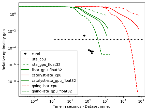
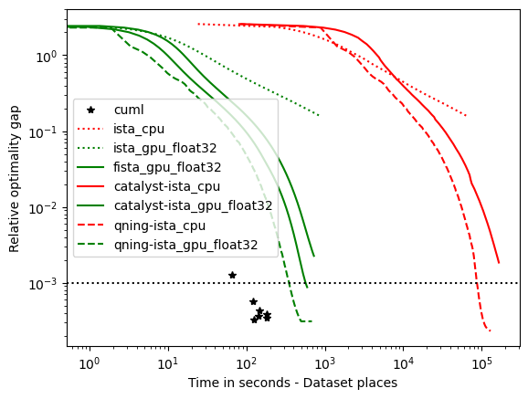
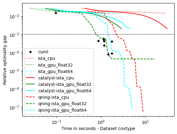
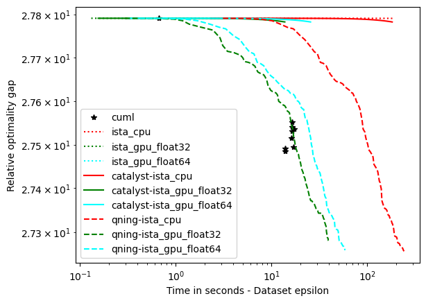
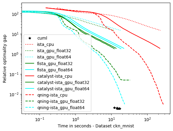
optimal \(\lambda\): covtype, epsilon, ckn_mnist – the hard ones

For these datasets, regularization is important, but not crucial to achieve a good predictive accuracy and thus the optimal \(\lambda\) is small. For instance, for ckn_mnist, the accuracy on test data is typically above 99%, and the dimension p for covtype is so small that regularization is useless. This leads to an interesting setting with clear conclusions.

Conclusions

• qning and catalyst accelerations are very useful. Note that catalyst works well in practice.

• The GPU version is at least 10 times faster than the CPU one. When we compare the two versions the GPU version is much faster, and we will see in the following part that bigger the dataset is bigger is the speed gap. (It is possible to almost reach a 100 times speedup)

• We can observe a significative difference for the solution depending on features datatype.

• Cyanure does better than sklearn-saga, lbfgs, and liblinear, sometimes with several orders of magnitudes. Note that sklearn-saga does as bad as our regular srvg solver for these dataset, which confirms that the key to obtain faster results is acceleration.

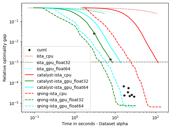
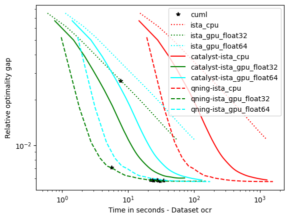
optimal \(\lambda\): alpha, rcv1, real-sim, ocr, kddb – the easy ones

For these datasets, the optimal regularization parameter is close to \(\frac{1}{n}\), which is a regime where acceleration does not bring benefits in theory. The results below are consistent with theory and we can draw the following conclusions:

• accelerations is useless here, as predicted by theory, which is why the ‘auto’ solver only uses acceleration when needed.

• qning-miso and catalyst-miso are still among the best solvers here, but the difference with svrg is smaller. sklearn-saga is sometimes competitive, sometimes not.